
Introduction
Production LLM serving systems were designed around a request model in which each request is self-contained. A request arrives carrying its full context, the model generates a response, and the request terminates. Contexts are small relative to device memory, and no per-request state needs to persist once generation completes. Existing systems exploit these properties throughout. Schedulers treat requests as interchangeable units of work, routers balance load without reference to request history, and the memory a request occupies is reclaimed at completion.
Agentic workloads violate each of these properties. An agent executes a task by iterating a reason-act loop. It produces a plan, invokes an external tool, consumes the result, and plans again. Every iteration is a distinct inference request that resubmits the task's accumulated context in full, and agents additionally spawn sub-agents that execute concurrently with the parent rather than after it. A single task therefore expands into hundreds of requests that are neither mutually independent nor uniformly spaced in time.
This shift relocates the dominant cost of serving. When the majority of a request's input has already been processed, the constraining resource is no longer compute but the KV cache that would have rendered the recomputation unnecessary. The design question is consequently not whether to retain that cache, but where it should reside, for how long, and how quickly it can be restored when a session resumes.
We address these questions empirically rather than analytically. The workload is not synthetic. We replay a public trace of production agent sessions request by request, preserving the recorded inter-request timings, token counts, and token cache block identities, and we report what retention buys, what its absence costs, and what the prefix cache must deliver.
Our findings reduce to three requirements. First, the KV cache must be retained, because recomputing it consumes the majority of available compute on work already performed and because reuse is certain to recur. Second, it must be shared, in the sense of being readable from whichever node serves a session's next request. A cache reachable only from the node that produced it forces the router to sacrifice either cache hit rate or cluster utilization. Third, the prefix cache must be fast, because a resuming request cannot begin execution until its entire context has been restored. The remainder of this post quantifies each requirement in turn.
TL;DR
- Agentic requests are large, nearly identical to the last one, and arrive together. Input outweighs output by 203 to 1, and 98.3% of that input is content the model has already processed. One session can put twenty-three requests in flight at once, because it spawns sub-agents that run beside the parent rather than after it.
- Retaining the KV cache is a requirement, not an optimization. Recomputing it instead of retaining it made TTFT 17 times worse and left each user with 2 output tokens per second where retaining it gives 28. How long it is retained sets how much has to be held, and about an hour captures essentially all of the benefit while a full day multiplies the per-node cache size by 7 times for 0.6 points of token hit rate.
- Retaining the cache is not enough. It has to be shared. A cache confined to the node that produced it forces the router to choose. Routing by load drops the per-request hit rate to 14% and cuts the output rate of every user on that node by 6.3 times, while routing by cache locality leaves the busiest node at 2.3 times the cluster mean and the rest of the cluster idle. A prefix cache every node can read is what lets the router balance load, and in our runs it sustained 4.8 times the load.
- Sharing the cache means moving it, so the read bandwidth of the shared prefix cache binds next. A returning request pulls its whole context at once, the 90th-percentile restore is 3 times the average one, and holding TTFT where users already experience it took 6.4 times the average read demand. Below that the tier does not degrade gently. Requests cross the client timeout, and an agentic application experiences that as failure rather than as slowness.
1. What agentic workloads demand
Agentic traffic has a recognizable shape, and four of its properties bear directly on the design of a serving system. Each one invalidates an assumption that conventional systems were built on.
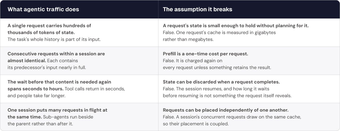
Two consequences follow, and the first is that retention ceases to be an optimization and becomes a requirement. Requests that are both large and nearly identical to their predecessors make holding a session's state cheaper than recomputing it, and the length of the wait means that state has to be held for a long and unpredictable duration. Taken together, the volume of KV that must remain live exceeds device memory, so it is offloaded to a tier below it. The design question therefore shifts from whether to retain the cache to where it resides and how quickly it can be restored.
The second consequence is that the cache has to be readable from whichever node takes the session's next request. Routing is otherwise no longer free to follow capacity, because placement and cache hit collapse into a single decision. Neither resolution of that decision works. Balancing load gives up the cache, and following the cache concentrates a session's requests on one node, since a session emits several of them at once. Making the cache readable everywhere separates the two decisions again and leaves the router free to place work wherever there is room.
So the core challenge of serving agentic traffic is not any one of these requirements but all three at once. The KV cache is too large to keep where it is fast, it is useless on a node that cannot read it, and it saves nothing if returning it takes as long as recomputing it. What the rest of this post measures is the cost of satisfying all three together.
2. Anatomy of the workload
The measurements in this post replay a public trace of production Claude Code sessions, captured through a proxy and released by SemiAnalysis as part of their InferenceX work. It records 393 sessions and 98,827 LLM calls carrying 21.6 billion input tokens, together with the per-request timings and cache block identities needed to reproduce prefix cache behavior. It is a recording of real usage rather than a synthetic benchmark, and every number below comes from it.
Requests are large, and successive ones are nearly identical
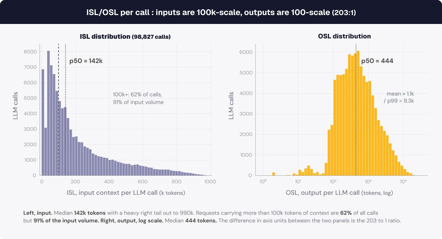
A session issues 251 LLM calls on average against a median of 86, with a heavy tail reaching 2,474 at the top percentile, and cumulatively submits 55.1 million input tokens. Each call carries 219k tokens of input against roughly a thousand tokens of output. The input volume is concentrated in the largest requests. Those above 100k tokens are 62% of the calls and carry 91% of the total input volume.
In the agentic trace, 98.3% of all input blocks have been read before. Only 1.7% is genuinely new, which is the ceiling on what any amount of caching can save. The session's unique content averages 931k tokens while its cumulative input is 42.6 times that. Recomputing the repeated part means most of the GPU is doing work it has already done, and this is the observation the rest of the post is built on. The obvious response is to keep the KV instead, and the difficulty is entirely in what happens next.
The wait before reuse spans seconds to hours
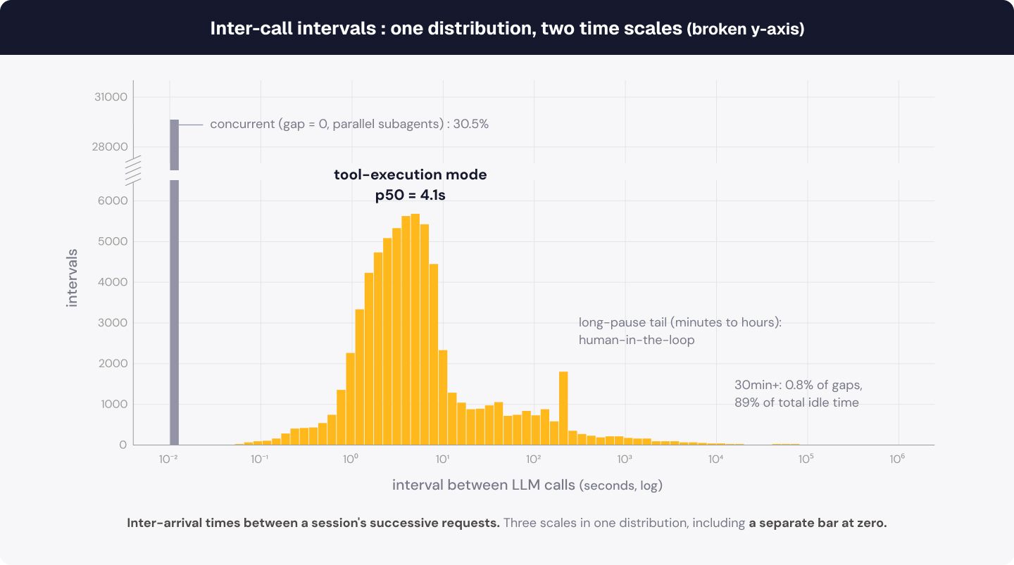
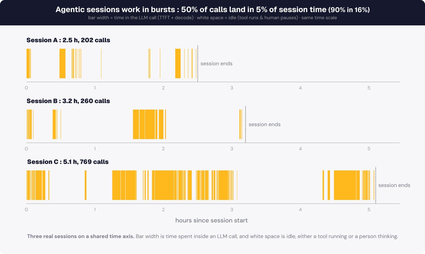
The inter-arrival time between a session's successive requests is multi-modal, and Figure 2 resolves three scales within it. Sub-agent concurrency produces intervals of zero, which are 31% of arrivals, because the request enters while the session is still occupied. Tool execution produces a mode measured in seconds, with a median of 4.1 s across the intervals in which the session was idle. Human-in-the-loop pauses produce a tail measured in minutes to hours, and that tail dominates the aggregate idle time, since intervals of thirty minutes or more account for 0.8% of arrivals but 89% of all idle time.
The same skew appears within an individual session. Requests arrive in bursts separated by idle intervals, and half of a session's requests fall within the busiest 5% of its minutes while ninety percent fall within 16%. A session is therefore active for a small fraction of its lifetime and idle for the remainder.
Together the two figures make the retention window a design parameter rather than a constant. Retaining a session's KV for its full lifetime removes the prefill from every subsequent request in that session, and pays for it by holding tens of gigabytes through pauses of hours in which nothing reads them. Retaining only what fits in device memory frees that capacity for other sessions, and pays for it by re-prefilling any session whose pause outlasts the space. Neither extreme is cheap in this workload, because the reuse is certain enough that early eviction wastes prefill work, and the tail is long enough that a window covering it holds capacity idle for hours. Choosing between the two is an operator policy rather than a property of the model or the hardware, and the infrastructure has to make that choice available.
A session puts many requests in flight at once
Those calls do not form a chain. Sub-agent groups appear in 44.5% of sessions, 1,697 groups in total at an average of 24.8 calls each, and although each group is mostly sequential inside itself, it runs alongside the parent conversation rather than in place of it. The consequence shows up directly in the concurrency. 95% of sessions have two or more calls in flight at some point, and one reaches twenty-three at once. A session is not one line of requests, and if its KV is bound to one place, that place has to absorb all of that concurrency by itself.
That is the problem this workload creates. The reuse is certain, the interval before it is not, and a session's concurrent requests all depend on the same state, so tens of gigabytes of KV per session has to survive an unpredictable wait and then come back fast enough that the user does not notice. Nothing in the chat-era stack was asked to do that.
3. KV has to be stored
Throughout this post a node is one eight-GPU server, and a cluster is the set of nodes a request can be routed across.
Per-token KV cost is falling and total KV is still growing
Attention design has moved deliberately toward smaller KV. Grouped-query attention reduced the number of key-value heads a token contributes, multi-head latent attention compresses each token into a low-rank latent, and sparse variants restrict how much of that state is attended to at each step. KV size is context length times the model's per-token KV footprint, so each of those steps lowers the first factor. The table below reports both factors at FP8 for four models spanning that progression, using the average LLM call in this trace, roughly 219k tokens of context, as the reference unit.
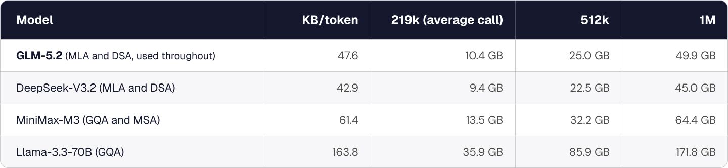
The per-token reduction is real and it is large. A token requires 163.8 KB on Llama-3.3-70B with grouped-query attention, 61.4 KB on MiniMax-M3, and 42.9 KB on DeepSeek-V3.2 with multi-head latent attention and a sparse indexer, a factor of 3.8 across that progression. Judged per token, the trend points in the direction an infrastructure designer would want.
Context length, however, has grown faster than the per-token cost has fallen. The average LLM call in this trace carries 219k tokens of context, so even the cheapest architecture in the table requires 9.4 GB of KV for a single call, and a one-million-token context on GLM-5.2 reaches 49.9 GB. Long reasoning traces and multi-turn sessions are what produce those lengths, and both continue to grow rather than converge. The KV that has to be stored is therefore still large, and it is still growing.
Retaining KV dominates recomputing it
Retention is not an optimization that trades latency for capacity. Discarding a session's KV when its request completes forces the next request to prefill its whole context again, which for the average call means computing 218,996 tokens instead of 3,700 and takes TTFT from 3.11 seconds to 52.4. The table shows what the two policies deliver on the same workload.

That waste repeats on every request of every session, so a node that keeps nothing spends its capacity recomputing context it has already computed. Both columns are measured on the same eight-node cluster and the same workload, so the difference between them is the retention policy and nothing else. Retaining KV also consumes less of the node, occupying a tenth of the utilization that recomputing requires.
How long it is kept sets how much has to be held
Retaining KV delivers a clear performance gain, but not everything can be retained, because retaining everything would mean storing 34 TB per node per day. A longer retention window raises the fraction of a request's context that is already resident, which lowers TTFT, and it simultaneously raises the volume that has to be held, because more sessions remain inside the window at once. How long KV is retained is therefore a choice rather than a value the hardware fixes, and that is what has to be decided.
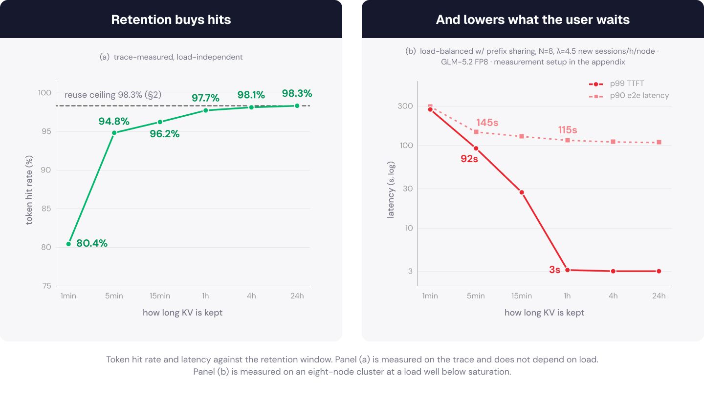
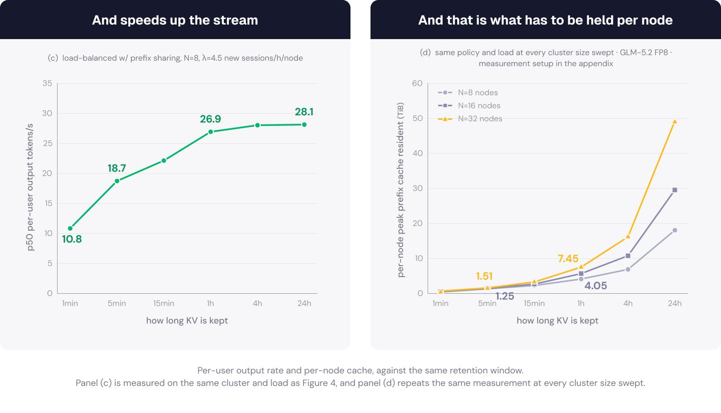
Performance and the resulting capacity requirement are measured against the retention window, from one minute to a day. Figure 4 (a) shows the token hit rate, rising steeply to five minutes and then approaching the workload's reuse ceiling. Figure 4 (b) shows p99 TTFT and the 90th-percentile end-to-end request latency, and Figure 5 (c) the per-user output rate, all three leveling off once the window reaches an hour. Figure 5 (d) shows the cache a node has to hold, which also grows with the number of serving nodes, because a session's requests spread across more of them and each node holds a copy of every session it has served. Retention therefore buys a saturating benefit at a cost that does not saturate. Both curves are set by the trace, so the window has to be decided against the workload a service actually serves.
Moving the window from five minutes to an hour adds only 2.9 points of token hit rate, but it takes p99 TTFT from 92 seconds to 3.1, raises the p50 per-user output rate by 1.44 times from 18.7 to 26.9 output toks/s, and improves the 90th-percentile end-to-end request latency by 1.26 times. Widening the window that far costs 4.9 times the per-node cache, and going from an hour to a day costs 6.6 times again while returning under five percent on both. Returns diminish beyond an hour, so on this trace an hour is the smallest window that still captures the tail, and its per-node cache requirement is 7.45 TiB.
The two windows compared here are the two that Anthropic's prompt caching exposes, a five-minute default and an optional one hour. Each use restarts the window from that point, so a window covers the interval between requests, not a session's lifetime. Read against Figure 2, the two settings line up with the two scales of that interval, five minutes covering the tool-execution loop and an hour reaching the pauses of a person working alongside the agent. Only 0.6 points of this workload's reuse requires an interval longer than an hour. Which of the two a service selects is a configuration decision, and the measurements above put a large performance difference between them.
4. KV has to be reachable from any node
The measurements in section 3 assume that a retained prefix is reachable from whichever node serves the next request. That assumption is not free. In a conventional deployment the KV a request produces stays in the node that produced it, so a session routed elsewhere finds nothing and prefills its context again. This section measures what the assumption is worth, which requires separating two decisions that a deployment normally makes together, how the router picks a node and where the KV lives.
A production router scores each node on how much of the request's prefix that node already holds and on how loaded it is, then sends the request to the best one. The two terms are weighted against each other inside one score, so affinity and load are settings on a dial rather than separate mechanisms, which is how both NVIDIA Dynamo and llm-d expose them. The three policies compared here take the two ends of that dial while the KV stays node-local, and then add a prefix cache that every node can read.

A router weighted on load sends each request to the least loaded GPU, and a router weighted on session affinity sends it to the GPU that already served that session. The first and third policies both use the load weighting and differ only in where the KV lives, which isolates the prefix cache. The second keeps the prefix cache node-local and routes for cache hits instead.
Each architecture is evaluated by raising the offered load, expressed as new sessions per hour per node, and recording where it stops meeting a service level. The service level used here is a 90th-percentile end-to-end request latency of 300 seconds. End-to-end latency rather than TTFT is the binding quantity, because an agent client applies its timeout to the whole request and a request that exceeds it fails rather than arrives late, while TTFT stays far below any documented client timeout. The 300 seconds is the per-request timeout default in OpenCode, a widely used coding agent. Clients that bound a whole agent turn instead, such as OpenClaw, carry a timeout default of 600 seconds, and while this post reports against the 300-second bar throughout, the same trend holds at 600 seconds.
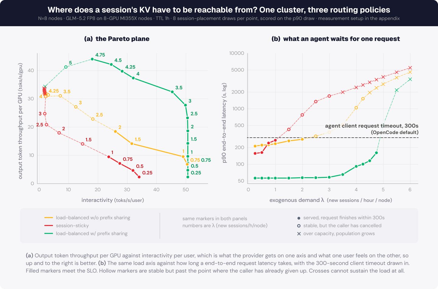
Under this service level the three architectures sustain very different offered loads. Routing by load over a shared prefix cache holds 4.75 new sessions per hour per node, against 2 for the same routing over a node-local prefix cache and 1 for session-sticky, which is 2.4 and 4.8 times the load. Neither shortfall comes from a lack of GPUs, and the two have different causes.
Session-sticky reaches a request hit rate of 99% and fails on placement. At the highest offered load it sustains, the busiest node runs at 2.33 times the cluster mean, while the other two policies stay within 1.06. The cause is the arrival shape measured in section 2, where a session is bound to one GPU and the sub-agent requests it issues concurrently can only go there. The imbalance is largest when the cluster is lightly loaded, reaching 3.37 times, since fewer sessions leave less to average over. The same failure mode is reported outside this work. llm-d writes that “the prefix-only scorer frequently overloaded replicas, succeeding in only ~55% of requests”, while “Prefix + Load maintained 100% success across all QPS levels”.
Routing by load over a node-local prefix cache balances work to within 2% of the shared architecture, but it fails on reachability. Its request hit rate is 14%, because routing by load scatters a session's requests across nodes while only the node that served it last holds its cache. The cost of those misses does not stay with the requests that missed. Prefills occupy slots until the mean per-GPU batch size climbs from 1.2 to 6.8, and requests sharing those slots slow with it, so the per-user output rate falls from 45 to 7 output toks/s with its tenth percentile from 28 to 5. Sub-agent fan-out amplifies this, since a session that issues twenty-three concurrent requests sends most of them to nodes that have to prefill its 219k-token context from nothing.
A prefix cache every node can read resolves both failures at once. Routing on load removes the imbalance and destroys the hit rate, and routing on affinity does the reverse, because a prefix only its producing node can read forces the router to choose between them. Figure 6 (a) shows what removing that choice is worth, with the shared architecture above and to the right of both alternatives at every operating point measured, producing 1.4 to 13.7 times the output tokens per GPU at the same speed per user. Raising utilization therefore cannot be solved by routing alone.
5. The shared tier has to be fast
Sharing a prefix means moving it. When a request hits a prefix held outside the node, vLLM keeps it out of the running batch until the transfer completes, and SGLang's hierarchical cache either waits for the prefetch or abandons the hit to avoid waiting. Either way the read bandwidth of the tier below sets how fast requests can enter execution, and therefore how much work the GPUs can be given. Sections 3 and 4 treat that path as free. This section places a shared storage cluster below the host DRAM cache and measures how much that cluster's access bandwidth changes the result.
The measurements below hold retention at the hour section 3 settled on and give each node 512 GB of host DRAM. That DRAM covers little of what is needed, because the working set of requests a node has in flight is measured in terabytes, so 86% of the KV that requests need comes from the shared tier and only 13% from local DRAM. Adding DRAM does not remove the bandwidth demand, it only moves where the demand is served.
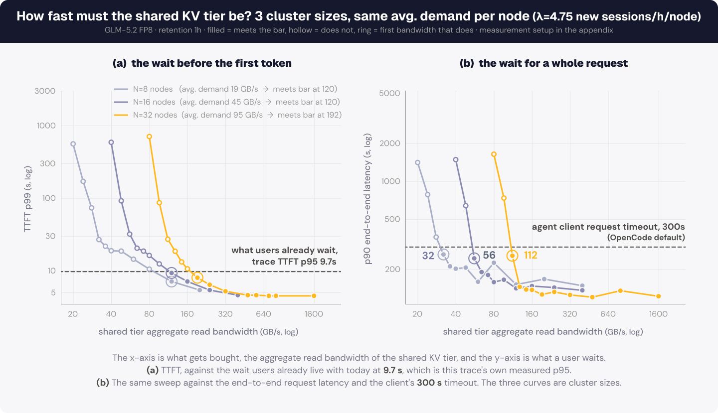
On the 8-node cluster the tier serves an average read demand of 19 GB/s, and the average is not what has to be provisioned. A returning request pulls its whole context in one read, 8.4 GB on average and 24.9 GB at the 90th percentile, so the tail read is 3.0 times the mean one. Figure 2 shows why those reads also arrive together, since 31% of the intervals between a session's successive requests are zero, meaning the next request starts while the session is still busy and its sub-agents read at the same instant. Holding the TTFT users already have therefore takes 120 GB/s, 6.4 times the average. Even end-to-end request latency, which is dominated by decode and moves little with the storage path, needs 32 GB/s, still 1.7 times the average. Neither criterion is met at the average, and bandwidth below them costs goodput and turns a slow read into an agent failure.
When the tier cannot absorb those bursts the failure reaches the agent rather than staying in the storage path. Cutting from 120 to 20 GB/s takes p99 TTFT from 7.4 to 560 seconds, past the 300-second client timeout of section 4, so those requests are cancelled rather than served late while the GPUs still look busy. Growing the cluster makes this more complex rather than smaller. One tier has to deliver 120 GB/s behind 8 nodes and 192 behind 32, for reads that cannot be late. As the cluster grows further the tier also stops being one uniform resource, because what a node can read depends on how it is attached. Serving agentic traffic well is therefore an infrastructure design problem, and what has to be designed is the path the KV travels.
6. Conclusion
Agentic requests carry large inputs and repeat nearly all of them, 219k tokens of context and 98.3% repetition, and they return after intervals ranging from zero to hours. A cluster that discards that state between requests cannot serve the load at all, so the KV has to be kept, and the retention window is what sets how much has to be held. Keeping it on the node that produced it forces the router to choose between placing work where there is room and placing it where the cache is, so a prefix cache every node can read is what lets a router balance load at all. Sharing it means moving it, so read bandwidth is the binding constraint, and a prefix cache that cannot deliver it drives agents into their client timeouts.
Classic inference infrastructure was built for requests whose state is small, short-lived and local to the GPU that produced it. Agentic traffic breaks all three at once, and what it exhausts first is not GPU compute but the capacity to hold KV and the bandwidth to move it. That is why agentic AI breaks classic inference infrastructure. A second post takes up what this one leaves out, the network that KV has to cross.
MangoBoost AIDC rack architecture
These requirements are what MangoBoost designs its AI data center (AIDC) racks around. In the reference architecture in Figure 8, every GPU compute node connects over 2x 200GbE to an Ethernet switch that fronts a layer of Mango Kesar™ storage controllers (KESAR-C). Each controller carries 4x 200GbE toward the compute nodes and 4x 200GbE toward its peer controllers, and reaches the KESAR-E enclosures behind a second switch over up to 8x 200GbE. Because every compute node reads from the same storage cluster, it serves as the shared prefix cache tier that sections 4 and 5 call for: reachable from any node, and provisioned for read bandwidth rather than capacity alone.
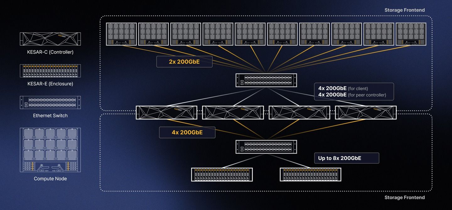
Every link in that diagram is a path the KV cache has to travel, and the fabric between compute and storage decides whether a shared prefix cache can return a session's context before the user notices. In our next post, we turn to that network and why it matters as much as the storage behind it.
Appendix. Simulation methodology
Every quantitative result in this post comes from MangoAIModel, MangoBoost's event-driven simulator for LLM serving on a multi-node cluster. It advances one engine iteration at a time per serving instance, so continuous batching, chunked prefill, prefix cache state and cross-node transfers are all resolved at the granularity the engine itself schedules at.
Iteration time is priced from a kernel library profiled on real GPUs rather than from an analytic performance model. The serving framework's own GEMM, attention, MLA and MoE kernels are executed on the target accelerator across a swept grid of shapes, and the simulator interpolates that grid to price each operator a batch issues. Prefill and decode times are assembled per iteration from the composition of the batch, since the shapes a step issues depend on how many requests are prefilling, how many are decoding and how long each context already is.
Collective communication is priced the same way, from RCCL and NCCL measurements taken on real GPUs over the real fabric. All-reduce, all-gather, reduce-scatter and all-to-all are swept over GPU count and message size on the target hardware, and the simulator interpolates those measurements for every collective an iteration issues. Inter-node transfers are priced from measured RDMA goodput rather than from nameplate line rate.
The resulting model was validated against real serving deployments before it was used here and holds within 10% over the range this workload occupies. That range is what agentic traffic makes demanding, contexts from a few thousand tokens up to one million and concurrency from a single request to the in-flight limit of a full node.
The serving software runs as real code rather than as a reimplementation of it, which makes these experiments a software-in-the-loop simulation. llm-d's router runs unmodified against simulator workers that present the model server interface it expects and publish KV cache events in its own wire format, so placement comes from llm-d's own scheduler and scorers rather than from a model of them. LMCache runs the same way, as the upstream package, supplying chunk hashing, lookup, tier promotion and eviction while the bytes those decisions move and the time they take stay modeled. Only GPU execution and the fabric are simulated.
References
Workload data
- SemiAnalysis InferenceX, cc-traces-weka-062126. huggingface.co/datasets/semianalysisai/cc-traces-weka-062126
Models and architecture
- vLLM, KV connector interface. docs.vllm.ai/en/stable/api/vllm/distributed/kv_transfer/kv_connector/v1
- SGLang HiCache, design and prefetch policies. docs.sglang.io/advanced_features/hicache_design
- NVIDIA Dynamo, KV cache aware routing. docs.nvidia.com/dynamo/latest/router/README.html
- llm-d, intelligent inference scheduling. llm-d.ai/blog/intelligent-inference-scheduling-with-llm-d
- Anthropic prompt caching, cache lifetimes. platform.claude.com/docs/en/docs/build-with-claude/prompt-caching
- GLM-5.2. huggingface.co/zai-org/GLM-5.2
- DeepSeek-V3.2. huggingface.co/deepseek-ai/DeepSeek-V3.2
- MiniMax-M3. huggingface.co/MiniMaxAI/MiniMax-M3
- MiniMax M3 in vLLM. vllm.ai/blog/2026-06-12-minimax-m3-vllm
- MiniMax Sparse Attention. arxiv.org/html/2606.13392v1
Serviceability bars
- OpenCode configuration. opencode.ai/docs/config
- OpenClaw agent configuration, timeouts. docs.openclaw.ai/gateway/config-agents
- Anthropic API errors. docs.anthropic.com/en/api/errors
Serving and KV tiering
- SGLang, DeepSeek usage and data parallelism attention. docs.sglang.io/basic_usage/deepseek_v3.html
- LMCache, KV cache management layer. docs.lmcache.ai
- SAC, CXL disaggregated KV for sparse attention. arxiv.org/pdf/2606.19746
Written by Advanced AI Team